Tutorial - Monte Carlo Simulation of self-assembly on Heterogeneous Surfaces: Fe-Terephthalate Ordering on Randomly Heterogeneous Cu(100) Surface

Here we provide a tutorial for the Monte Carlo simulation of the self-assembly of two-dimensional metal–organic network on randomly heterogeneous surface. We consider the Fe–Terephthalate ordering on the Cu(100) with point defects. In this example, we use the parallel tempering Metropolis Monte Carlo scheme in grand canonical ensemble.

Model

We used the lattice model of TPA–Fe/Cu(100) adsorption monolayer presented in our paper [1]. A square lattice with parameter a is used as a model of Cu(100) surface. According to the experimental data [2], TPA molecules and Fe atoms are adsorbed in hollow sites on the Cu(100) surface. As a model of a heterogeneous Cu(100) surface we have chosen the surface with a random distribution of point defects. The defects describe holes (the absence of a copper atom in the crystal structure), atom displacements (dislocations), impurities, etc. Thus, TPA molecules and Fe atoms can be adsorbed on the defect and hollow adsorption site in our model.

Please download the archive TPA_Fe_heterogeneous_Cu100.zip Here you can find xyz-files with adsorption complexes of TPA and Fe and pair configurations called samples, as well as energy file specifying the energy values for each pair configuration.

A series of ordered metal–organic structures consisting of TPA molecules and Fe atoms are formed on Cu(100) surface [2]. We have distinguished two representative phases among all of them. The “cloverleaf” phase consists of metal atoms coordinating four TPA molecules. Hydrogen bonding between molecules also involved in the formation of the structure. The “single-row” phase is formed by the “– TPA – 2Fe –” chains perpendicular to each other. This phase is stabilized only by TPA–Fe coordination interactions.

A key parameter of the model is energetic heterogeneity \(\Delta\) of the surface. It is a difference between the adsorption energies on the defect and hollow adsorption site. This value has positive sign if the adsorption on hollow site is more preferred than adsorption on the defect. Otherwise, it is negative.

Code for Monte Carlo Simulation

Please download the following script TPA_Fe_heterogeneous_Cu100.py and read below what the script does.

import numpy as np
from susmost import *
from susmost.mc import *
from susmost import mc
from mpi4py import MPI
from math import exp
from time import time
from susmost.mc import make_regr, tmatrix

# Conditions for the single-row phase (C): muTPA = 25, muFe = 25.
# Conditions for the cloverleaf phase (B): muTPA = 10, muFe = 42.
# Fadeeva A.I. et al. // J. Phys. Chem. C. 2019. Vol. 123, № 28. P. 17265.

lt = load_lattice_task('TPA_Fe_heterogeneous_Cu100')

lt.set_property('coverage', {'TPA':1, 'Fe':1})
lt.set_property('TPA_cnt', {'TPA':1, 'gTPA':1})
lt.set_property('Fe_cnt', {'Fe':1, 'gFe':1})
lt.set_property('He_cnt', {'gCu':1, 'gTPA':1, 'gFe':1})

print (lt.states)

muTPA = 10.0
muHe = 0
muFe = 42.0
Lx = 24     # lattice size
Ly = 24
delta = 5   # energetic heterogeneity parameter, kJ/mol
T_list = [300., 500., 700., 900.]   # K

lt.set_ads_energy('TPA', muTPA) # kJ/mol
lt.set_ads_energy('Fe', muFe)   # kJ/mol
lt.set_ads_energy('gTPA', muTPA + delta)        # kJ/mol
lt.set_ads_energy('gFe', muFe + delta)  # kJ/mol
lt.set_ads_energy('gCu', muHe)  # kJ/mol

D = 0.1     # fraction of defects
defect_sites = np.random.permutation(Lx*Ly)[:int(Lx*Ly*D)]

m = mc.make_metropolis(lt, (Lx, Ly), T_list, 0.00831)   # R=0.00831 kJ/(mol*K)
m.transitions = tmatrix.make_tmatrix_with_fixes(lt.states, 'He_cnt', fixed_prop_diff=0)

if MPI.COMM_WORLD.Get_rank() == 0:
        m.lattice.load_cells('cells_cloverleaf_24x24')
        for i in defect_sites:
                m.cells[i] = 4
        bcast_data = m.cells
else:
        bcast_data = None

m.cells[:] = MPI.COMM_WORLD.bcast(bcast_data,root=0)

l = run (m, log_periods_cnt = 20, log_period_steps = 1000*Lx*Ly, relaxation_steps = 500000*Lx*Ly, traj_fns=["muTPB={}_muCu={}_T={}_D={}.xyz".format(muTPA, muFe, T, D) for T in T_list])
stat_digest(m)

The load_lattice_task function generates the lattice model from the provided xyz-files of the adsorption complexes and pair configurations, and interaction and energy files specifying the types and values of the pair interaction energies in the model.

The lt.set_property function states a properties of interest for the model. Here, lt.set_property('TPA_cnt', {'TPA':1, 'gTPA':1}) sets the counter for the adsorbed TPA molecule both on a defect and hollow adsorption site equal to 1. It means one molecule per lattice site. The same meaning carries the line lt.set_property('He_cnt', {'gCu':1, 'gTPA':1, 'gFe':1}), but for the amount of the defects on the lattice. It is seen that amount of defects is independent of the site occupation. A defect site can be empty or occupied be the TPA molecule or Fe atom, the 'He_cnt' equals 1 for all states of the defected site. Note that here we have identified a point defect in the form of a hollow site with pre-adsorbed helium atom. Remind, the name of each adsorption complex is included in the head of the corresponding xyz-file. For example, you may see ac_name=TPA in the top of the adsorbate_state_2.xyz and adsorbate_state_3.xyz files.

muTPA, muFe and muHe are the state energies of the isolated TPA, Fe adsorption complexes and the defect site, in kJ/mol. Physical meaning of state energy μ is the energy change caused by formation of the corresponding adsorption complex on a clean surface. Lx and Ly values specify the linear size of the lattice in a units along the x and y directions, respectively. delta is the energetic heterogeneity parameter \(\Delta\), in kJ/mol. It has the same value for the TPA molecules and Fe atoms in our model. In this example, the \(\Delta\) value has the same order as the lateral interactions in our model. T_list is a list of temperatures in Kelvins for parallel tempering Monte Carlo simulation.

The lt.set_ads_energy function sets the state energies of the adsorption complexes. The state energy for an occupied site is set equal to the \(\mu\) value. In the case of adsorption on a defect, we also add the value of the energetic heterogeneity parameter to this energy. D is the fraction of surface defects. For example, D = 0.1 means that we have 10% surface defects. The function np.random.permutation randomly distributes the selected number of defect sites over the surface of a given size.

The make_metropolis function creates a task m for Monte Carlo simulation. The tmatrix.make_tmatrix_with_fixes function modifies the m.transitions transition matrix, which defines the allowed transitions from between all the site states in the model, in such a way that some transitions are prohibited. Here, the tmatrix.make_tmatrix_with_fixes(lt.states, 'He_cnt', fixed_prop_diff=0) function fixes the position of the defects on the surface. It declares that property 'He_cnt' for each site should not change during the simulation. Therefore, the defects are not displaced during the simulation.

In this example we wish to simulate the effect of surface defects on the thermal stability of particular ordered structures observed experimentally in the TPA-Fe/Cu(100) metal-organic layer. Therefore, we should construct the wished molecular structure on the defected lattice before the simulation. If you start the simulation with an empty surface, you do not have to do that. Just star the simulation as usually.

The next part of the code loads the ideal lattice state for each metal-organic structure from the “cells_cloverleaf_24x24”, “cells_singlerow_24x24” files, modifies it setting defect sites and broadcasts it to all parallel replicas. These lattice state files have been saved during the simulation of the same model on the homogeneous Cu(100) surface (see Example of Model of Fe-Terephthalate Ordering on Cu(100) : Monte Carlo method).

So, please download the prepared lattice state files for both phases cells_cloverleaf_24x24, cells_singlerow_24x24. The provided files fit the lattice with the linear size equal to 24. The loading of the lattice states can be done during the simulation by using the m.lattice.load_cells function. To set the defect sites, the state number corresponding to the defect state need to be specified. The numbers of the site states in the considered lattice model are included in the name of the corresponding “adsorbate_state_{index}.xyz” files. There are 3 states of the site in the model on the homogeneous surface, namely 0 for empty site, 1 – for the site occupied by the Fe atom, 2 and 3 - for the site occupied by the TPA molecule in two perpendicular orientations. In the considered heterogeneous model there are another for states: 4 – for the empty defect, 5 – for the defect occupied by the Fe atom, 6 and 7 – for the defect site occupied by the TPA molecule. You may also see it in your command window once you run the script due to the presence of print (lt.states) line in the code. Thus, we should set the state “4” to the defect sites from the defect_sites list.

Further, we run the m simulation with relaxation time – 500 000 Monte Carlo steps (MCS), plus 20 000 MCS for thermal averaging over the 20 points. Every 1000 MCS in the production run we save the xyz-snapshots having 20 snapshots at the end of the simulation at each considered temperature. stat_digest prints summary on sample statistics.

Note that the unzipped “TPA_Fe_heterogeneous_Cu100.zip” folder, “mc_TPA_Fe_get_Cu100.py” and “cells_cloverleaf_24x24”, “cells_singlerow_24x24” files must be located in the same directory.

Please start a Monte Carlo simulation specifying 4 MPI processes (equal to the number of temperatures indicated in the code).

Results

Fig. 1 shows the typical result of the Monte Carlo simulation of the cloverleaf phase on a Cu(100) surface with point defects. The phase was obtained at the chemical potentials of TPA molecules and Fe atoms equal to 10 and 42 kJ/mol, respectively.

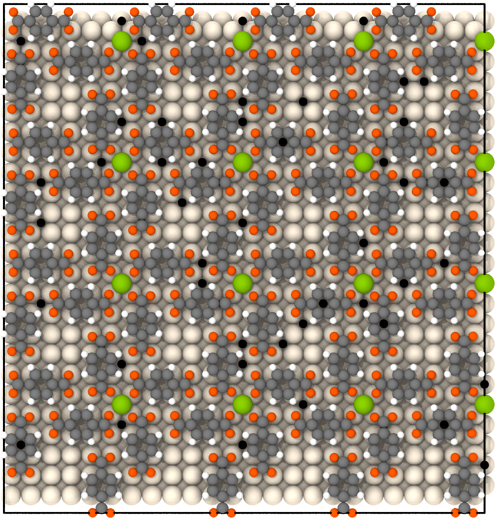
Fig. 1. Cloverleaf phase in the Fe-Terephthalate adlayer on a heterogeneous Cu(100) surface at \(\mu_{TPA} = 10\) kJ/mol and \(\mu_{Fe} = 42\) kJ/mol. Lattice size is 24×24 and temperature is 300 K.

In Fig. 2 you can see the simulated single-row phase at the following chemical potentials of the components: \(\mu_{TPA} = 25\) kJ/mol and \(\mu_{Fe} = 25\) kJ/mol.

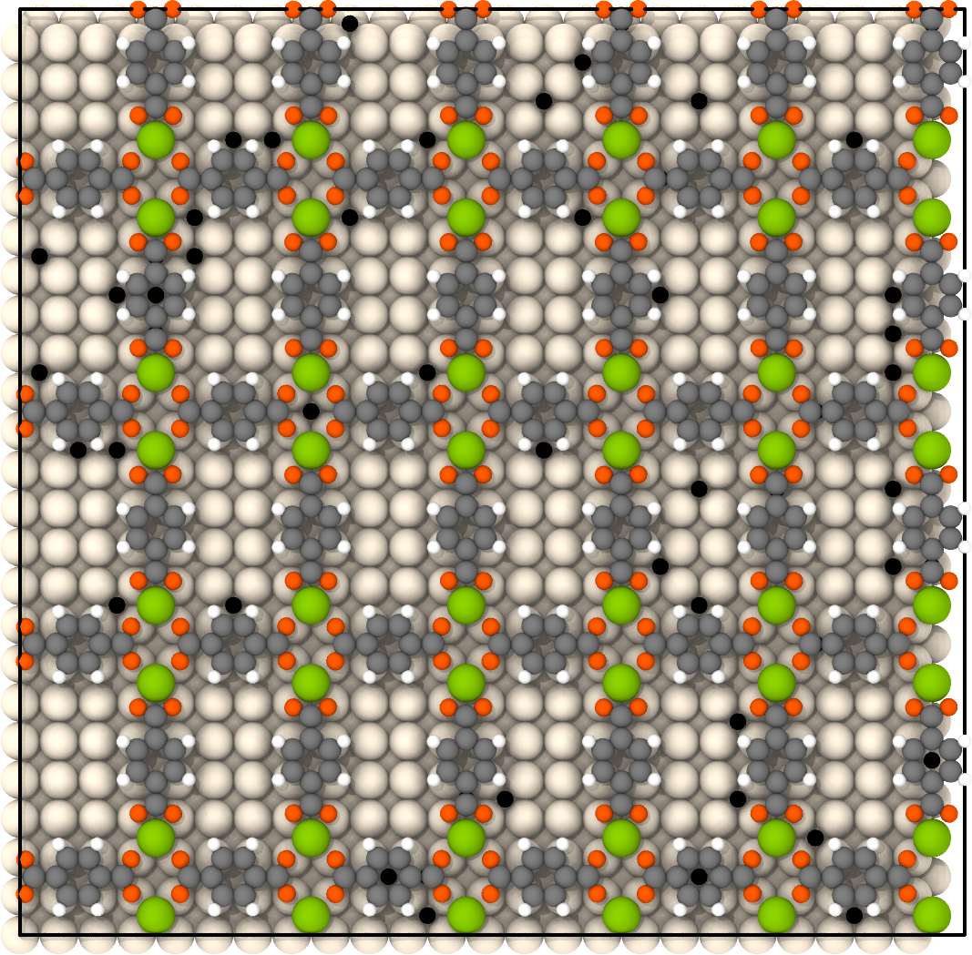
Fig. 2. Single-row phase in the Fe-Terephthalate adlayer on a heterogeneous Cu(100) surface at \(\mu_{TPA} = 25\) kJ/mol and \(\mu_{Fe} = 25\) kJ/mol. Lattice size is 24×24 and temperature is 300 K.

Fig. 3 demonstrates the dependence of the layer heat capacity on the temperature calculated at the bigger lattices, namely 48x48 and 144x144. Please see how to calculate the heat capacity in the tutorial Monte Carlo simulation additive binary gas mixture.

The peaks on the heat capacity curves indicate the melting temperatures of the considered metal-organic structures.

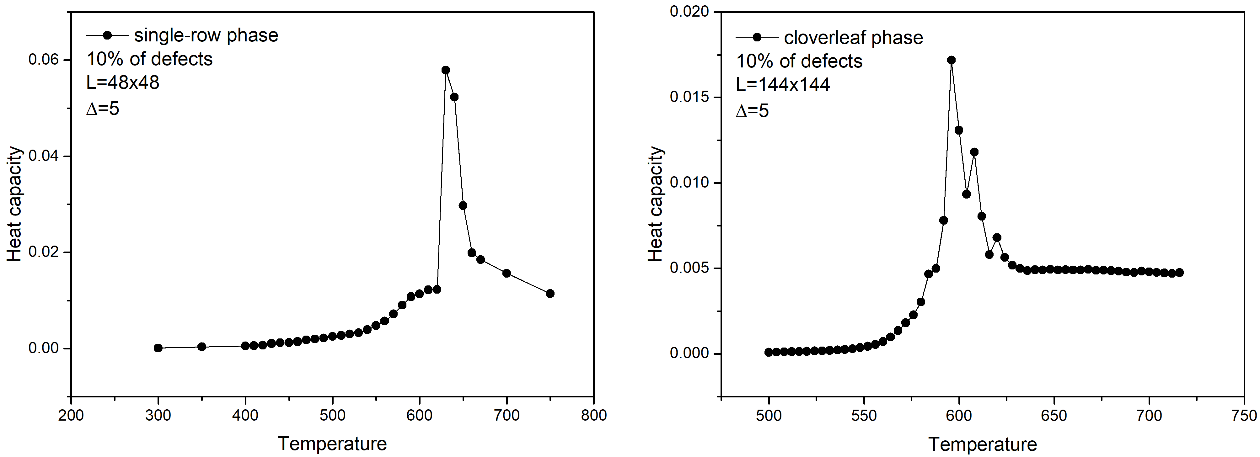
Fig. 3. Heat capacity vs. temperature calculated for the single-row (left) and cloverleaf (right) phases.

References

[1]

A.I. Fadeeva, V.A. Gorbunov, P.V. Stishenko, A.V. Myshlyavtsev, Model of Fe-Terephthalate Ordering on Cu(100), J. Phys. Chem. C. 123 (2019) 17265–17272. https://doi.org/10.1021/acs.jpcc.9b02834.

[2]

M.A. Lingenfelder, H. Spillmann, A. Dmitriev, S. Stepanow, N. Lin, J.V. Barth, K. Kern, Towards Surface-Supported Supramolecular Architectures: Tailored Coordination Assembly of 1,4-Benzenedicarboxylate and Fe on Cu(100), Chemistry - A European Journal. 10 (2004) 1913–1919. https://doi.org/10.1002/chem.200305589.