Tutorial - Transfer-matrix simulation additive binary gas mixture

In this tutorial we provide an example of applying the Transfer-matrix method to simulate the adsorption of additive binary gas mixtures on solid surfaces. The additive gas mixture means that lateral interactions have been introduced between the adsorbed particles for each component of the gas mixture. In this tutorial we use SUrface Science MOdeling and Simulation Toolkit (SuSMoST)

Please have a look at the following script here and read below what the script does.

Libraries

In this block we include libraries. Here numpy is standard library. susmost is a general library that contains modules required for setting structure of model and applying the Transfer-matrix method.

import numpy as np
from susmost import make_single_point_zmatrix, make_square_plane_cell, \
        normal_lattice_task, transferm, SiteStateType, register_property, \
        sitestate, nearest_int, make_tensor, solve_TM

Constants

Here we define the constants.

INF_E  = 1E6
k_B = 8.3144598E-3
a = 1.0
r_cut_off= 8.0 + .0001

In the table below, we show the constants and their descriptions.

Constant	Description
INF_E	Prohibitive energy level
k_B	Gas constant, kJ/(mol*K)
a	Lattice constant
r_cut_off	Parameter required to calculate the transfer-matrix

Note

If k_B is measured in kJ/K, then k_B is the Boltzmann constant .

Parameters

Here we define the parameters.

N = 6
T = 100.0
eAA = 4.
eBB = 6.
dop_int = {('mol_A','mol_B'):0.0,('mol_A','mol_A'):eAA,('mol_B','mol_B'):eBB}
interaction = lambda cc1,cc2: nearest_int(cc1,cc2,dop_int=dop_int)

In the table below, we show the parameters and their descriptions.

Parameter	Description
N	Width of the semi-infinite system (infinite in one direction and finite in perpendicular one)
T	Temperature, K
eAA	Interaction energy A-A, kJ/mol
eBB	Interaction energy B-B, kJ/mol
dop_int, interaction	Interaction energy between neighbor sites of the lattice depending on their states, kJ/mol

Here we set the lattice geometry that models the solid surface.

cell,atoms = make_square_plane_cell(a)
    register_property('coverage_A','==', None, sitestate.join_cover)
    register_property('coverage_B','==', None, sitestate.join_cover)

In this models we use a square lattice with lattice parameter a (make_square_plane_cell(a) and etc.). The lattice constant a specifies the location of the nodes. We set the properties of each node (coverage_A, coverage_B).

Initial data

In this block we initialize input data. Here mus - array of chemical potential differences in the gas and adsorption layer \(\mu_g - \mu_a \approx-RTlnp\), covs - array of coverages, \(\beta=1/(k_B T)\).

beta = 1./(k_B*T)
mus = []
covs = []

Calculation of coverages

Set interval in what we change the pressure in the gas phase. molA_state, molB_state and empty_state specifies the shape of the nodes (make_single_point_zmatrix()), sets the energy of adsorption for each state of the lattice site (molecule A - muA, molecule B - muB, empty - 0), assigns the mark to all the possible surface states (molecule A - atom N, molecule B - O, empty - H), sets the properties of each node (molecule A - coverage=1., coverage_A=1., coverage_B=0., molecule B - coverage=1., coverage_A=0., coverage_B=1., empty - coverage=0., coverage_A=0., coverage_B=0.).

The lattice model description is stored in lt as objects of the class LatticeTask.

Set W as a tensor of interaction that can be used to solve eigenvalue problem [1] (read more: interface round a face [2] ), avg_cov is the average cover corresponding to each ring (where avg_cov is the total average cover, avg_covA and avg_covB are the average covers by A and B molecules) and tm_sol as solution of transfer-matrix.

In result we’ll get an array of the calculated coverages by transfer-matrix method covs (where cov is the total coverage, covA and covB are the fractional coverages by A and B molecules) and the chemical potential mus.

for muA in np.arange(-20., 20.+0.0001, 2. ):
            molA_state = SiteStateType('mol_A', make_single_point_zmatrix(), muA, ['N'],
                                    coverage=1., coverage_A=1., coverage_B=0.)
            molB_state = SiteStateType('mol_B', make_single_point_zmatrix(), 0.0, ['O'],
                                    coverage=1., coverage_A=0., coverage_B=1.)
            empty_state = SiteStateType('Empty',make_single_point_zmatrix(), 0.0, ['H'],
                                    coverage=0., coverage_A=0., coverage_B=0.)

            lt = normal_lattice_task([molA_state, molB_state, empty_state], cell, atoms, interaction, r_cut_off, INF_E)

            W = make_tensor(lt, beta)

            avg_cov = transferm.average_props(lt.states, N, 'coverage', beta)
            avg_covA = transferm.average_props(lt.states, N, 'coverage_A', beta)
            avg_covB = transferm.average_props(lt.states, N, 'coverage_B', beta)

            tm_sol = solve_TM(W, N, symmetric=True)

            cov = sum(tm_sol.probs*np.array(avg_cov))
            covA = sum(tm_sol.probs*np.array(avg_covA))
            covB = sum(tm_sol.probs*np.array(avg_covB))
            covs.append([cov, covA, covB] )
            mus.append(muA)
            print ("muA ==", muA, "theta == ",cov)

Results

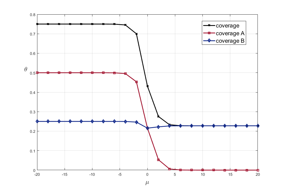
In the Fig.1 the fractional surface coverages with molecules A and B, and the total surface coverage are shown as functions of the chemical potential of the molecules A in the adlayer. It is worth to note that the equivalence of the chemical potentials in gas phase and in the adlayer is supposed. Therefore, the lower values of the chemical potential of the molecule A in the adlayer, the higher pressure of the gas A in the gas phase mixture.