Tutorial - Monte Carlo simulation additive binary gas mixture
Here we provide an example of applying the Monte Carlo method to simulate the adsorption of additive binary gas mixtures on solid surfaces [1]. The additive gas mixture of two components means that lateral interactions are considered only for the adsorbed molecules of the same type. For example, the binary system of A and B components is described by thwo types of lateral interactions: A-A and B-B, but not A-B.
Lattice Gas Model
Please download the model Binary_gas_mixture.zip.
As a model of the surface we use the square lattice with a distance between nearest neighbor sites.
See the sample_empty_unit_cell.xyz file. There are three state of the adsorption site in this model.
They are set up in the following xyz-files: adsorbate_state_0.xyz, adsorbate_state_1.xyz and adsorbate_state_2.xyz
for an empty site, for a site occupied with A molecule and molecule B. All states in the model
are represented by monomeric spherical particles. We assign a mark to all the possible surface states
(molecule A - atom N, molecule B - O, empty - H). The name of the state in each xyz-file can be
found in the head of the corresponding file. The above mentioned lateral interactions between A-A, A-B and B-B molecules
are specified in the energy file and equal to 4.0, 0.0 and 6.0 kJ/mol, respectively.
Please also download the following script mc_binary_gas.py and read below what the script does.
lt = load_lattice_task('./')
lt.set_property('coverage', {'A':1.0, 'B':1.0} )
lt.set_property('A_cnt', {'A':1})
lt.set_property('B_cnt', {'B':1})

L = 36 # lattice size
T = 100. # K
muB = 0.
lt.set_ads_energy('B', muB) # kJ/mol
kB = 0.008314 # kJ/(mol*K)
Function load_lattice_task load the lattice model into the SuSMoST.
Here we also define some properties of the site states such as coverage
that equal to 1 for both A and B adsorption complexes, and zero (by default) for
an empty site. A_cnt and B_cnt are for the amount of A and B adsorption complexes on the lattice.
Also we are setting up the key constants and model parameters:
Lis the linear size of the lattice inaunits;Tis the temperatures in the adsorption layer;muBis the chemical potential of the B component that is set bylt.set_ads_energyequal to the state energies of the B adsorption complexes.
as
lt.set_ads_energywe set the state energies of the available adsorption complexes aslt.set_ads_energy. Note that in this tutorial, the chemical potential of the componentsmuAandmuBmeans the differences between molar Gibbs free energy of the component in the gas phase and adsorption layer \(\mu_{Bgas} - \mu_{Bads} \approx-RTlnp_B\). The chemical potential of the A component will be varied in the simulation, so it will be set up further.
kBis Gas constant in kJ/(mol*K). Ifk_Bis measured in kJ/K, thenk_Bis the Boltzmann constant .
Set the Monte Carlo Simulation
Here we perform the Monte Carlo simulation of the model in Grand Canonical Ensemble for a given amount of Monte Carlo steps at fixed values of the B component chemical potential and temperature, changing the chemical potential of the A molecules.
# Perform the simulation for a series of TEtB chemical potentials

for mu in np.arange(30., 0.-0.0001, -2.0 ):
        lt.set_ads_energy('A', mu)    # kJ/mol
        m = mc.make_metropolis(lt, L, temperatures, kB)
        mc.run(m, log_periods_cnt=10, log_period_steps = 1000*m.cells_count, relaxation_steps = 100000*m.cells_count, \
                traj_fns = ["T={}.xyz".format(T) for T in temperatures])
Here we run the m simulation for each value of the chemical potential of the A component in the range from 20 to -30 kJ/mol with step of -2 kJ/mol.
Each time we set new value of the A component chemical potential using lt.set_ads_energy.
make_metropolis function creates a task m for Monte Carlo simulation. Here we perform 100 000 Monte Carlo steps (MCS) for the system relaxation
and 50 000 MCS for thermal averaging over the 50 points.
Recall that MCS is the amount of attempts to switch the state of the lattice equaled to the amount of the lattice sites.
Every 1000 MCS in the production run we save the xyz-snapshots having 50 snapshots at the end of the simulation at each value of the muA.
It takes about 25 min on an average CPU.
Calculation the thermodynamic averages
We have obtained as simple averages the total (H) and potential energy (U) of the adlayer per lattice site,
the total surface coverage (coverage), partial coverage of the surface with A (A_cnt) and B (B_cnt) molecules
at the temperature 100 K changing the chemical potential of the component A from 20 to -30 with step = -2 kJ/mol.
Also we have calculated the differential heat of adsorption (Qd) and heat capacity (C).
All averages are calculated using 50 points. Results are saved in file.
E_2 = 0
covE = 0
cov_2 = 0
for T, param_log in zip(temperatures, m.full_params_log):
        stat = np.mean(param_log,axis=0)[[0, -2, -3]] # coverage, H, U
        for log_row in param_log:
                E_2 += log_row[-3]**2.0
                covE += log_row[0]*log_row[-3]
                cov_2 += log_row[0]**2.0
        E_2 /= len(param_log)
        covE /= len(param_log)
        cov_2 /= len(param_log)
        Qd = -(covE - stat[0]*stat[2])/(cov_2-stat[0]**2.0)
        Cp = (L^2)*(E_2 - stat[2]*stat[2])/(T*T*kB)
where
E_2is the squared total energy per lattice site;
covEis the value of surface coverage multiplied by potential energy;
cov_2is the squared coverage;
Qdis the differential heat of adsorption calculated with equation [3]\[Q_{d} = \frac{\langle\theta \cdot E\rangle-\langle \theta \rangle \cdot \langle E \rangle}{\langle \theta^2 \rangle-{\langle \theta \rangle}^2}\]
Cis the heat capacity of the molecular layer calculated as [4]\[C = L^2 \cdot \frac{\langle H^2 \rangle-\langle H \rangle^2}{T^2 R}\]
Results
In the Fig.1 the fractional surface coverages with molecules A and B, and the total surface coverage are shown as functions of the chemical potential of the molecules A in the adlayer. It is worth to note that the equivalence of the chemical potentials in gas phase and in the adlayer is supposed. Therefore, the lower values of the chemical potential of the molecule A in the adlayer, the higher pressure of the gas A in the gas phase mixture.
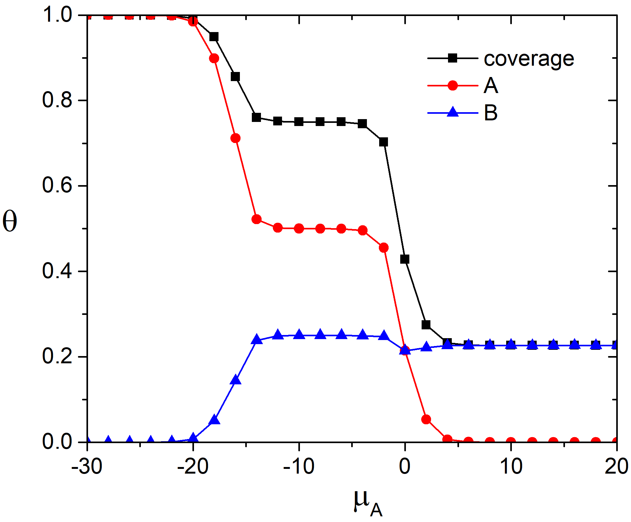
Fig. 1. Total and partial adsorption isotherms at 100 K and \(\mu_{B} = 0\) kJ/mol and \(e_{AA} = 4\) kJ/mol, \(e_{BB} = 6\) kJ/mol.
Animation on the Fig.2 illustrates the loading of the adlayer with increase of the chemical potential of A component.
Fig. 2. Loading of the adsorption layer with \(\mu_{A}\) increasing at 100 K and \(\mu_{B} = 0\) kJ/mol and \(e_{AA} = 4\) kJ/mol, \(e_{BB} = 6\) kJ/mol.
As it is well-known heat capacity of the system has a peak in vicinity of the phase transition. Dependence of the heat capacity of the adlayer on the chemical potential of the molecules A is shown in the Fig. 3. We can see there are few pronounced peaks on the heat capacity curve. They correspond to the continuous phase transitions those related to an appearance or disappearance of a symmetry element [5].
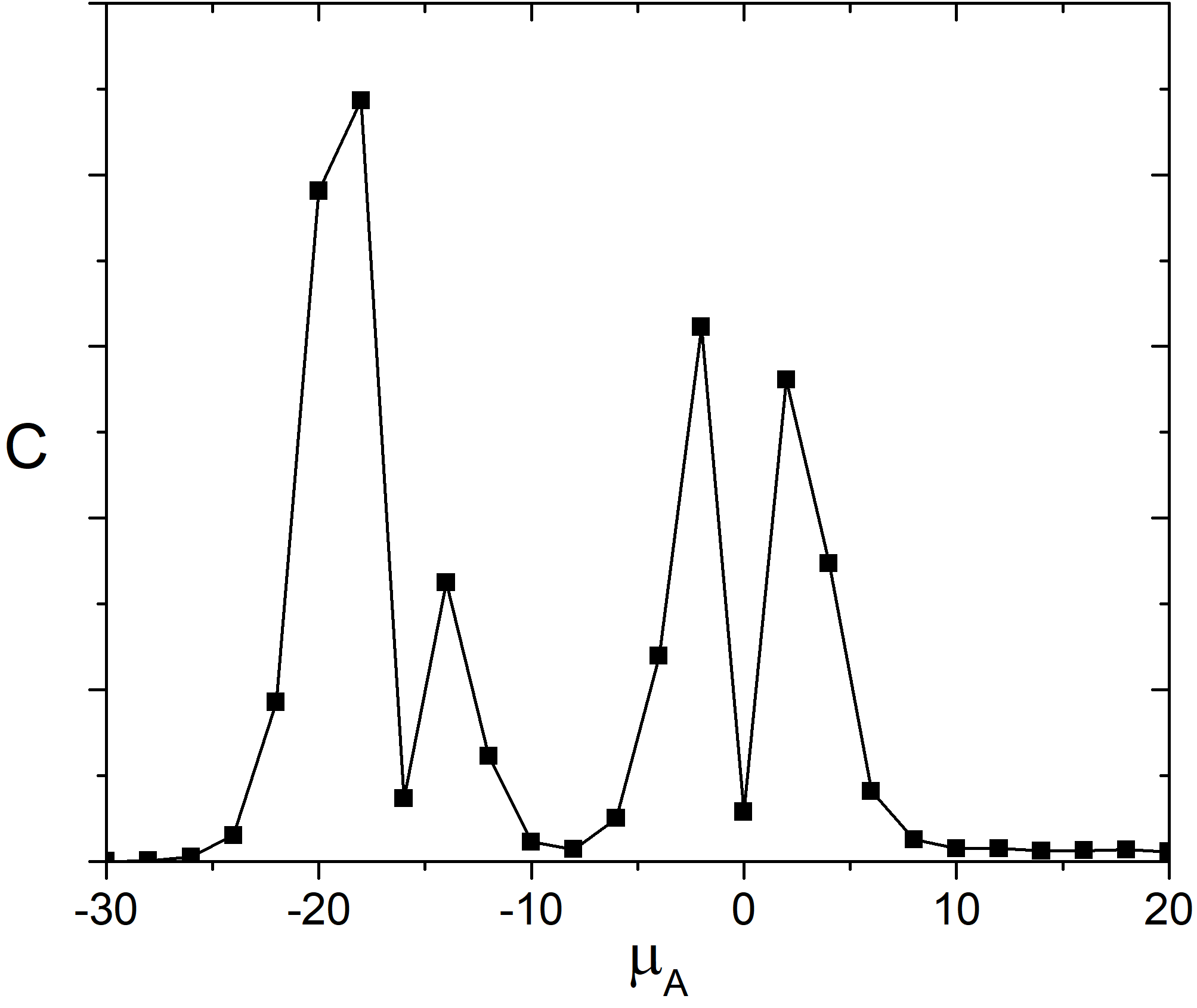
Fig. 3. Heat capacity of the adlayer vs. \(\mu_{A}\) at 100 K and \(\mu_{B} = 0\) kJ/mol and \(e_{AA} = 4\) kJ/mol, \(e_{BB} = 6\) kJ/mol.
Detailed discussion of this and other results on adsorption of the binary gas mixture can be found in the papers [1] and [2].