Tutorial - Monte Carlo simulation of the Langmuir adsorption model with nearest neighbor interactions
In this tutorial we provide an example of applying the Monte Carlo method as implemented in SuSMoST to simulate the Langmuir adsorption model with interaction between nearest neighbors.
Please have a look at the following script mc_langmuir.py and read below what the script does.
Libraries
In this block we include libraries. Here numpy and mpi4py are standard libraries. load_lattice_task and mc are the modules of the susmost general library required for setting up the structure of the lattice model and applying the Monte Carlo methods to simulate that.
from susmost import load_lattice_task
from susmost import mc
import numpy as np
from mpi4py import MPI
Constants, Parameters and Model
Please download the archive Langmuir_model.zip,
where all files needed for the model definition are provided.
Here we exploit the following assumption of the Langmuir adsorption model:
- All adsorption sites are equivalent (assume the surface is homogeneous);
Each site can hold at most one molecule of A (mono-layer coverage only).
As a model of the surface we use the square lattice with a distance between nearest neighbor sites.
See the sample_empty_unit_cell.xyz file. Only two xyz-files for adsorption complexes are available. They are
adsorbate_state_0.xyz and adsorbate_state_1.xyz for empty and occupied states of the site, respectively.
In this example we take into account the interaction between molecules adsorbed at nearest neighbor sites.
Therefore, there is a single pair configuration sample_001.xyz with non-zero interaction energy.
The value of such interaction is provided in the energy file.
lt = load_lattice_task('./')
lt.set_property('coverage', {'occupied':1.0} )
L = 60                  # lattice size
temperatures = [400, 500, 700, 1000]    # K
kB = 0.008314   # kJ/(mol*K)
Function load_lattice_task load the lattice model into the SuSMoST.
lt.set_property states the property coverage for the adsorption complex named “occupied” equal to 1.
Note that name of the adsorption complex is included in the head of the corresponding xyz-file. In this case,
you may see ac_name=occupied in the top of the adsorbate_state_1.xyz file.
Also we are setting up the key constants and model parameters:
Lis the linear size of the lattice inaunits;temperaturesis a list of temperatures for parallel tempering Monte Carlo simulation;kBis Gas constant in kJ/(mol*K). Ifk_Bis measured in kJ/K, thenk_Bis the Boltzmann constant .
Setting Up the Monte Calo Simulation
Here we perform the Monte Carlo simulation of the Langmuir model with interaction between nearest neighbors
in Grand Canonical Ensemble for a given amount of Monte Carlo steps at fixed
values of chemical potential and different temperatures, see temperatures.
Firstly, we set the state energies of the available adsorption complexes as lt.set_ads_energy.
The state energy of an empty site is assumed to be zero, so we ignore it. And the state energy for
an occupied site is set equal to the chemical potential mu. Note
that in this tutorial, the chemical potential mu means the differences between molar Gibbs
free energy of the gas phase and adsorption layer \(\mu_g - \mu_a \approx-RTlnp\).
for mu in np.arange(20., -80.-0.0001, -5.0 ):
# for mu in np.arange(30., 0.-0.0001, -2.0 ):
        lt.set_ads_energy('occupied', mu)       # kJ/mol
        m = mc.make_metropolis(lt, L, temperatures, kB)
        mc.run(m, log_periods_cnt=10, log_period_steps = 1000*m.cells_count, relaxation_steps = 100000*m.cells_count, \
                traj_fns = ["T={}.xyz".format(T) for T in temperatures])
        mc.stat_digest(m)
make_metropolis function creates a task m for Monte Carlo simulation.
Here we run the m simulation for each value of the chemical potential
with relaxation time - 100 000 Monte Carlo steps (MCS) and 10 000 MCS for thermal averaging over the 10 points.
Recall that MCS is the amount of attempts to switch the state of the lattice equaled to the amount of the lattice sites.
Every 1000 MCS in the production run we save the xyz-snapshots having 10 snapshots at the end of the simulation at each considered temperature.
stat_digest prints summary on sample statistics.
Calculation the thermodynamic averages
We have obtained as simple averages the potential energy of the adlayer and the surface coverage at fixed temperatures (400, 500, 700, 1000 K) changing the chemical potential:
from 20 to -80 with step = -5 kJ/mol for the repulsive interaction between nearest neighbors (\(\epsilon = 10\) kJ/mol);
from 30 to 0 with step = -2 kJ/mol for the attractive interaction between nearest neighbors (\(\epsilon = -5\) kJ/mol).
Also we have calculated the differential heat of adsorption and heat capacity. All averages are calculated using 10 points. Results are saved in file.
E_2 = 0
covE = 0
cov_2 = 0
for T, param_log in zip(temperatures, m.full_params_log):
        stat = np.mean(param_log,axis=0)[[0, -2, -3]] # coverage, H, U
        for log_row in param_log:
                E_2 += log_row[-3]**2.0
                covE += log_row[0]*log_row[-3]
                cov_2 += log_row[0]**2.0
        E_2 /= len(param_log)
        covE /= len(param_log)
        cov_2 /= len(param_log)
        Qd = -(covE - stat[0]*stat[2])/(cov_2-stat[0]**2.0)
        Cp = (L^2)*(E_2 - stat[2]*stat[2])/(T*T*kB)
where
E_2is the squared potential energy per lattice site;
covEis the value of surface coverage multiplied by energy;
cov_2is the squared coverage;
Qdis the differential heat of adsorption calculated with equation [1]
Results
Fig.1 shows typical results of the simulation of the Langmuir model with the repulsive interactions between nearest neighboring particles. On the A and C panel we can see the adsorption isotherms and heat capacities vs. the chemical potential calculated at different temperatures. There are three plateaus on the isotherms those correspond to lattice gas, chess-like and close-packed phases of the adlayer. Two peaks of the heat capacity are related to the phase transitions from the lattice gas to chess-like structure and further transition to the close-packed monolayer. The differential heat of adsorption and potential energy of the molecular layer as functions of surface coverage are shown on the panels B and D. Stable phases of the adlayer are revealed as steps on the differential heat curves and inflection points on the potential energy curves.
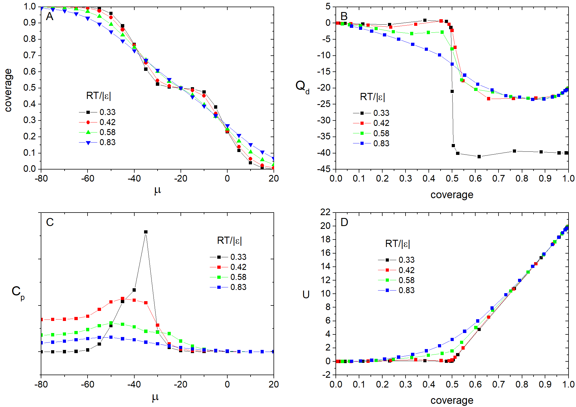
Fig. 1. Results of the simulation at \(\epsilon = 10\) kJ/mol.
The animations of the adsorption layer with decrease of the chemical potential (increase of the gas phase pressure) at 400 K and 1000 K are shown in the Fig. 2 and Fig.3.
Fig. 2. Filling the monolayer at \(RT/\epsilon = 0.33\).
Fig. 3. Filling the monolayer at \(RT/\epsilon = 0.83\).
Fig.4 and Fig. 5 demonstrates a behavior of the adlayer with attractive interactions between nearest neighbors \(\epsilon = -5\) kJ/mol at different temperatures \(RT/|\epsilon| = 0.66\) and \(RT/|\epsilon| = 1.66\) with increase of the gas phase pressure. A surface condensation as the first order phase transition occurs in the adlayer only at the low temperature. At the high temperature, for example \(RT/\epsilon = 1.66\), the close packed phase appears as a result of continuous filling of the surface when the gas phase pressure increases.

Fig. 4. Filling the monolayer at \(RT/|\epsilon| = 0.66\).

Fig. 5. Filling the monolayer at \(RT/|\epsilon| = 1.66\).
The adsorption isotherms and heat capacity as a function of the chemical potential of the adlayer calculated at various temperatures are shown in the Fig.5A and Fig.6C, correspondingly. It is seen that the isotherms at high temperatures are smooth, but have the step at lower ones. The heat capacity tends to infinity in the point of the first order phase transition, which we observed at low temperatures. At high temperatures there is only a finite step on the heat capacity. And it disappears with further increasing of temperature. The Fig.6B,D represent the behavior of the potential energy and differential heat of adsorption vs. surface coverage.
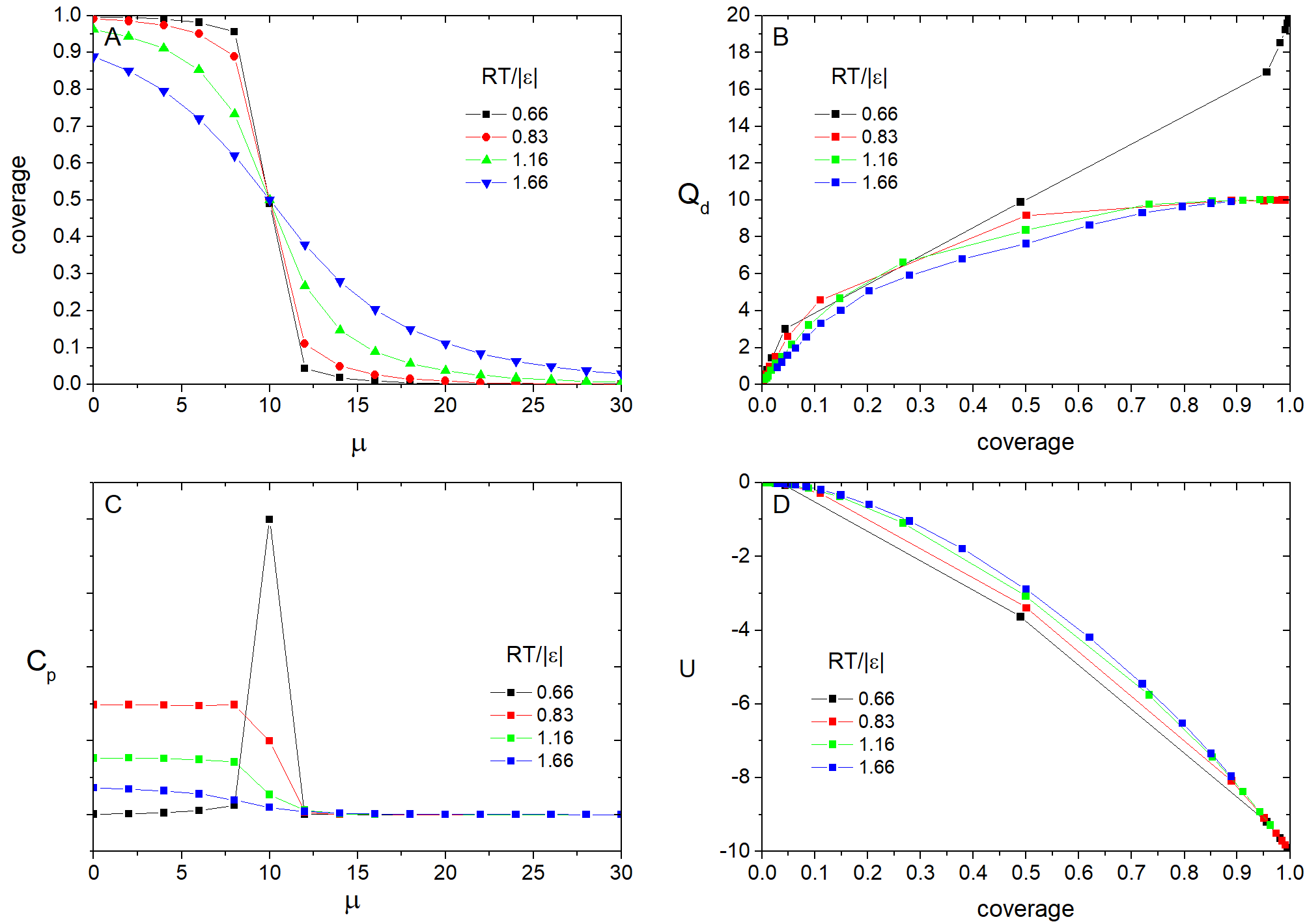
Fig. 6. Results of the simulation at \(\epsilon = -5\) kJ/mol.