Running simulations
To run simulations with SuSMoST one needs
Python interpreter with installed SuSMoST Python packages
An adsorption model
A Python script with simulation code
SuSMoST Python packages installation is described in Installing SuSMoST. Adsorption models are essentially directories with several files. They can be downloaded from the Downloads page, or found in a models directory of SuSMoST installation. Most of models included in SuSMoST contains example.py scripts with exemplar simulation code.
The simplest simulation script (NH3/V3C2 model)
For example lets try to do simulation for the NH3/V3C2 model. First of all lets activate SuSMoST’s Python environment:
$ source ve/bin/activate
Then change your current directory to the model’s directory:
$ cd models/NH3-V3C2
Then launch the example.py script:
$ python example.py
If everything has been done right, in some second you will see the output:
2.7487196394264197
This is a natural logarith of the model’s partition function per site. If you are interested in details, take a look at the source of the example.py script.
Along with the simple example.py script the NH3-V3C2 directory also contains more complicated and usefull example-isotherm.py. It prints out surface coverages for a sequence of NH3/V3C2 adsorption complex energies:
-0.3 0.9554971864503797
-0.24 0.8563763324198087
-0.18 0.7513212340924432
-0.12 0.6294038161599375
-0.06 0.5028657967144572
0.0 0.3445965667110924
0.06 0.1522997166803156
0.12 0.028102706082451023
0.18 0.0030560681307699716
0.24000000000000005 0.00030207886450439256
0.3 2.9554309932887306e-05
Here is an isotherm plot from these data:

The simplest simulation script with MPI (CO/Pt(111) model)
Simulations scripts that use parallel tempering algorithm should be launched appropriately. An example of such script is the example.py file in CO/Pt(111) model. To launch this script you need activate Python environment with SuSMoST and set working directory to the model directory, just like in previous example:
$ source ve/bin/activate
$ cd models/CO-Pt111
But you need to launch such scripts via mpiexec command with number of processes that is equal to number of parallel replicas requested by the script. Number of replicas correspond to the lenght of temperatures list that is passed to the :py:func:make_metropolis function. The models/CO-Pt111/example.py script requests four temperatures, hence it should be launched in this way:
$ mpiexec -n 4 python example.py
Successfull simulation should print out statistical digest about simulation. Like this:
Temperature # 0 = 2.0
        Parameter # 0 : 'coverage'
                Sample size      1000
                Sample mean     0.307809
                Sample stdDev   0.000183
                Autocorrelation function parameters:
                        First zero time:         30
                        Exponential time:       10.556 (RMSE=0.038)
                        Integrated time:        27.107
                Effective sample size integrated        36.891
                Effective sample size exponential       47.366
                Sample mean stdDev      0.000
        Parameter # -2 : 'Energy'
                Sample size      1000
                Sample mean     -0.003104
                Sample stdDev   0.000000
                Autocorrelation function parameters:
                        First zero time:         24
                        Exponential time:       8.418 (RMSE=0.054)
                        Integrated time:        14.961
                Effective sample size integrated        66.839
                Effective sample size exponential       59.399
                Sample mean stdDev      0.000
        Correlations between parameters:
                 1.000 0.865
                 0.865 1.000
Temperature # 1 = 8.965331703353698
        Parameter # 0 : 'coverage'
                Sample size      1000
                Sample mean     0.306266
                Sample stdDev   0.001398
                Autocorrelation function parameters:
                        First zero time:         66
                        Exponential time:       16.284 (RMSE=0.030)
                        Integrated time:        23.136
                Effective sample size integrated        43.223
                Effective sample size exponential       30.704
                Sample mean stdDev      0.000
        Parameter # -2 : 'Energy'
                Sample size      1000
                Sample mean     -0.003090
                Sample stdDev   0.000006
                Autocorrelation function parameters:
                        First zero time:         93
                        Exponential time:       26.992 (RMSE=0.028)
                        Integrated time:        35.761
                Effective sample size integrated        27.964
                Effective sample size exponential       18.524
                Sample mean stdDev      0.000
        Correlations between parameters:
                 1.000 -0.694
                 -0.694 1.000
Temperature # 2 = 10.695830923113437
        Parameter # 0 : 'coverage'
                Sample size      1000
                Sample mean     0.304536
                Sample stdDev   0.002205
                Autocorrelation function parameters:
                        First zero time:         49
                        Exponential time:       11.973 (RMSE=0.040)
                        Integrated time:        12.767
                Effective sample size integrated        78.325
                Effective sample size exponential       41.762
                Sample mean stdDev      0.000
        Parameter # -2 : 'Energy'
                Sample size      1000
                Sample mean     -0.003076
                Sample stdDev   0.000010
                Autocorrelation function parameters:
                        First zero time:         101
                        Exponential time:       24.256 (RMSE=0.027)
                        Integrated time:        28.377
                Effective sample size integrated        35.240
                Effective sample size exponential       20.613
                Sample mean stdDev      0.000
        Correlations between parameters:
                 1.000 -0.615
                 -0.615 1.000
Temperature # 3 = 12.0
        Parameter # 0 : 'coverage'
                Sample size      1000
                Sample mean     0.302917
                Sample stdDev   0.002512
                Autocorrelation function parameters:
                        First zero time:         42
                        Exponential time:       10.671 (RMSE=0.042)
                        Integrated time:        12.250
                Effective sample size integrated        81.634
                Effective sample size exponential       46.855
                Sample mean stdDev      0.000
        Parameter # -2 : 'Energy'
                Sample size      1000
                Sample mean     -0.003066
                Sample stdDev   0.000012
                Autocorrelation function parameters:
                        First zero time:         63
                        Exponential time:       17.843 (RMSE=0.036)
                        Integrated time:        21.985
                Effective sample size integrated        45.485
                Effective sample size exponential       28.022
                Sample mean stdDev      0.000
        Correlations between parameters:
                 1.000 -0.667
                 -0.667 1.000
Recommended temperatures: [2.0, 8.119878894794397, 10.375217380314396, 12.0]
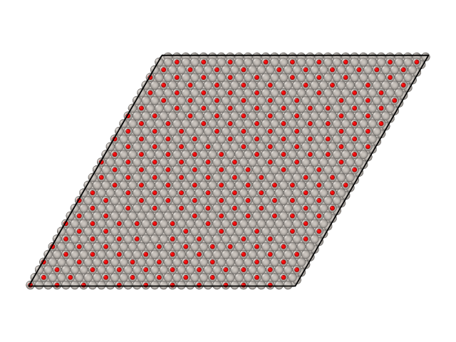
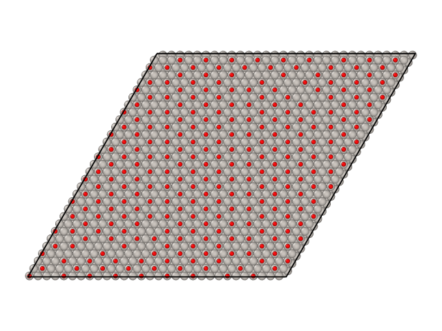
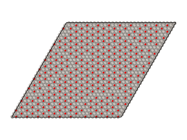
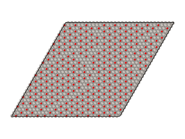
Parallel tempering simulations also generate surface samples as XYZ files. By default these samples are stored in files named traj_T.xyz, where T is the temperature of the sample. Here are samples from CO/Pt(111) simulations we ran above.
|
|
|
|