Tutorial - Transfer-matrix simulation Langmuir adsorption model with interaction

In this tutorial we provide an example of applying the transfer-matrix method to the Langmuir adsorption model with interaction between nearest neighbors. SUrface Science MOdeling and Simulation Toolkit (SuSMoST) is a set of computer programs and libraries that are used for modeling. As a result of the program, we get adsorption isotherm \(\theta(\mu)\).

Please have a look at the following script here and read below what the script does.

Libraries

In this block we include libraries. Here numpy is standard library. susmost is a general library that contains modules required for setting structure of model and applying the Transfer-matrix method.

import numpy as np
from susmost import make_single_point_zmatrix, make_square_plane_cell, \
        normal_lattice_task, transferm, nearest_int, SiteStateType, make_tensor, solve_TM

Constants

Here we define the constants.

INF_E  = 1E6
k_B = 8.3144598E-3
a = 1.0
r_cut_off= 8.0 + .0001

In the table below, we show the constants and their descriptions.

Constant	Description
INF_E	Prohibitive energy level
k_B	Gas constant, kJ/(mol*K)
a	Lattice constant
r_cut_off	Constant required to calculate the transfer-matrix

Note

If k_B is measured in kJ/K, then k_B is the Boltzmann constant .

Parameters

Here we define the parameters.

N = 8
T = 200.0
mol_int = 2.5

In the table below, we show the parameters and their descriptions.

Parameter	Description
N	Width of the semi-infinite system (infinite in one direction and finite in perpendicular one)
T	Temperature, K
mol_int	Interaction energy, kJ/mol

Here we set the lattice geometry that models the solid surface.

cell,atoms = make_square_plane_cell(a)
interaction = lambda cc1,cc2: nearest_int(cc1,cc2,mol_int)

In this models we use a square lattice with lattice parameter a (make_square_plane_cell(a) and etc.). The lattice constant a specifies the location of the nodes. interaction define an interaction between neighbor sites.

Initial data

In this block we initialize input data. Here mus - array of chemical potential differences in the gas and adsorption layer \(\mu_g - \mu_a \approx-RTlnp\), covs - array of coverages, \(\beta=1/(k_B T)\).

beta = 1./(k_B*T)
mus = []
covs = []

Calculation of coverages

Set interval in what we change the pressure in the gas phase. mono_state and empty_state specifies the shape of the nodes (make_single_point_zmatrix()), sets for each node the energy of adsorption ( monomer - mu, empty - 0), assigns the mark to all the possible surface states (monomer - atom N, empty - H), sets the properties of each node (monomer - coverage=1., empty - coverage=0.).

The lattice model description is stored in lt as objects of the class LatticeTask.

Set W as a tensor of interaction that can be used to solve eigenvalue problem [1] (read more: interface round a face [2] ), avg_cov - the average cover corresponding to each ring and tm_sol as solution of transfer-matrix.

In result we’ll get an array of the calculated coverages by transfer-matrix method covs and the chemical potential mus.

for mu in np.arange(-30., 20.+0.0001, 2.0 ):
        mono_state = SiteStateType('mono', make_single_point_zmatrix(), mu, ['N'], coverage=1.)
        empty_state = SiteStateType('Empty',make_single_point_zmatrix(), 0.0, ['H'], coverage=0.)

        lt = normal_lattice_task([mono_state, empty_state], cell, atoms, interaction, r_cut_off, INF_E)

        W = make_tensor(lt, beta)

        avg_cov = transferm.average_props(lt.states, N, 'coverage', beta)
        tm_sol = transferm.solve_TM(W, N, symmetric=True)

        cov = sum(tm_sol.probs*np.array(avg_cov))
        covs.append(cov)
        mus.append(mu)
        print ("mu ==", mu, "theta == ", cov)

Examples

Let’s look at some examples of using the application by varying input data, such as:

energy of interaction mol_int;
step of adsorption energy mu;
temperature T.

Note

We considered examples for the width of the lattice N=6. In case of necessary it can be changed too.

Example 1.

Assume we have next initial data:

Data
T = 100
mu = (-50,50,1)

here step_mu=1.

Let change the value of interaction energy mol_int. As result we get the following adsorption isotherms (fig. 1)

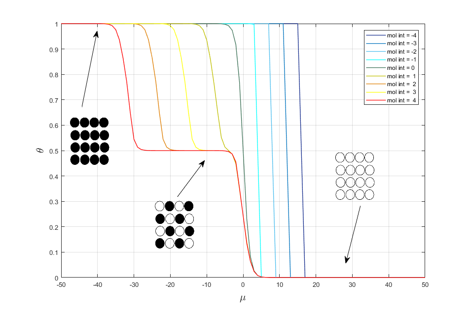
Fig. 1. Adsorption isotherms for different interaction energy.

It is seen from fig. 1 that in case of attraction we get the two-dimensional condensation and in the case of repulsion we get two phase transitions with forming of a chess and dense phases. If mol_int = 0, then we get classical Langmuir model.

Example 2.

Assume we have next initial data:

Data
T = 100
mol_int = 4
mu = (-10,10)

Let change the step of adsorption energy mu. As result we get the following adsorption isotherms (Fig. 2)

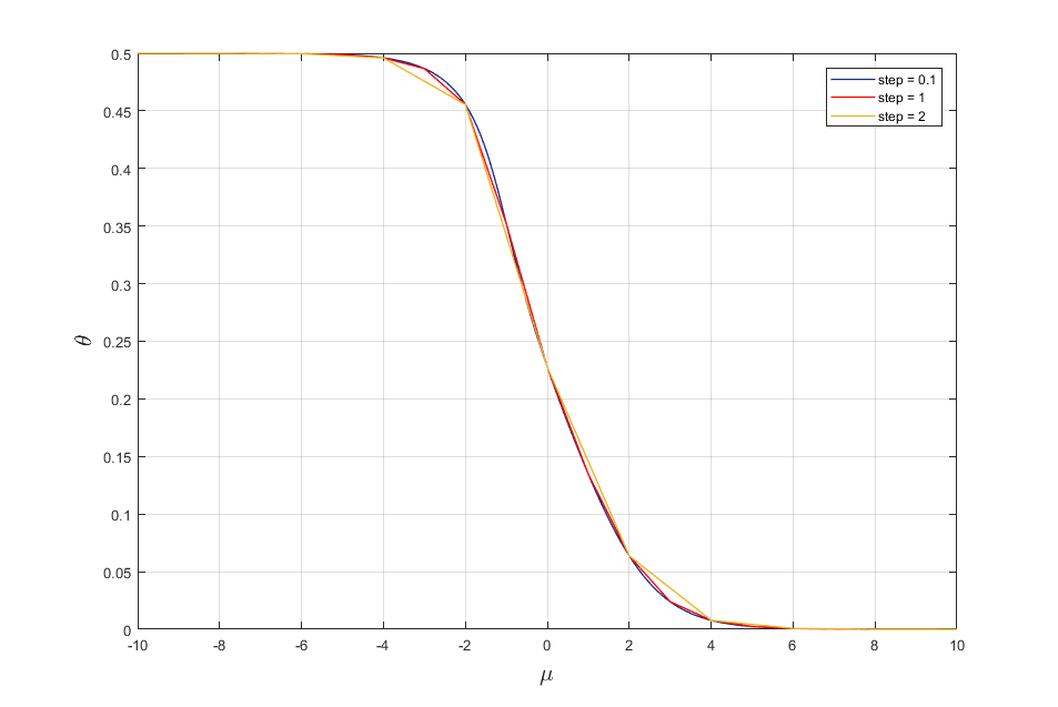
Fig. 2. Adsorption isotherms for mu = (-10,10) with different step.

It is seen from fig. 2 that by changing the step of adsorption energy mu we can obtain adsorption isotherms with a certain accuracy.

Example 3.

Assume we have next initial data:

Data
mu = (-50,50,1)
mol_int = 4

Let change values of temperature T. As result we get the following adsorption isotherms (Fig. 3)

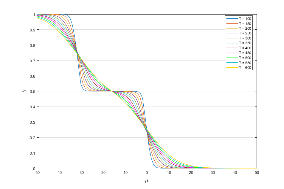
Fig. 3. Adsorption isotherms for different values of temperature.

It is seen from fig. 3 that with increasing temperature the region of existence of the phases are reduced to their disappearance.